S696, Maps and Atlases: The Cambridge Map Room

I’ve re-entered the academic world as a student at the University of Cambridge in the United Kingdom, and one of the benefits I’m enjoying the most is near-unlimited access to one of the world’s largest repositories of recorded information; the Cambridge University Library. Commonly known as the UL, this is a copyright library which means that under British rules on legal deposit, the library has the right to request a copy of any work published in the UK free of charge. Currently, the UL has over 8 million items, which includes books, periodicals, magazines and of course, maps.


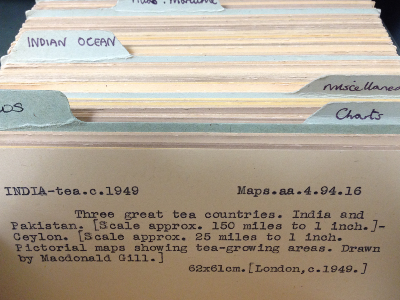
The Map Room in the UL is a fascinating place; it functions as the reading room for the Map Department, which holds over a million maps (as the librarian told me; Wikipedia claims it has 1.5 million). It’s not a very large room, as reading rooms go, but is a beautiful space and is very well managed. Everything is catalogued very efficiently with a filing card system, and there’s one card with the name, date of publication and classmark (UID/coordinates) for each map.  Visitors are not allowed to simply browse through the map collections; to refer to a map, one must fill out a request form with the appropriate details and submit this form to the library assistants, who will then pull out the required map folio from its storage location. The title of this post comes from the fact that  map holdings with classmarks beginning with ‘S696′, ‘Maps’ or ‘Atlases’ are held in the Map Room, in various drawers and cabinets.

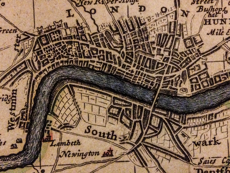
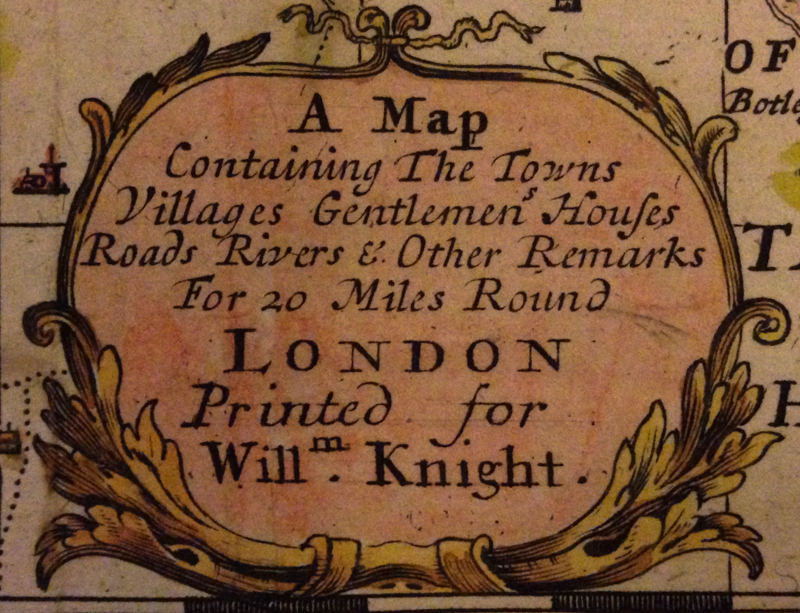
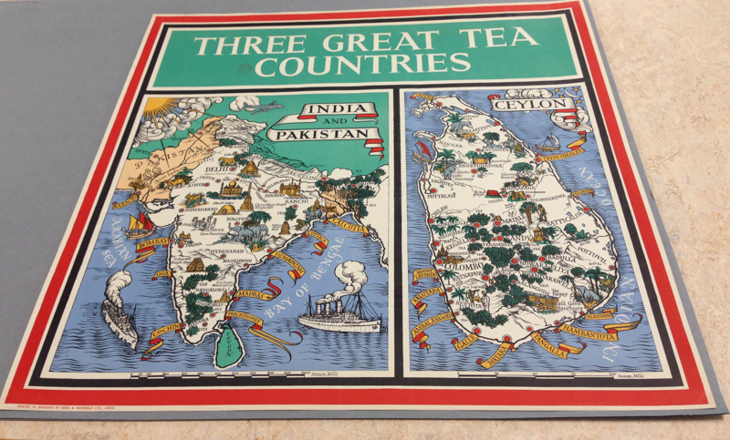
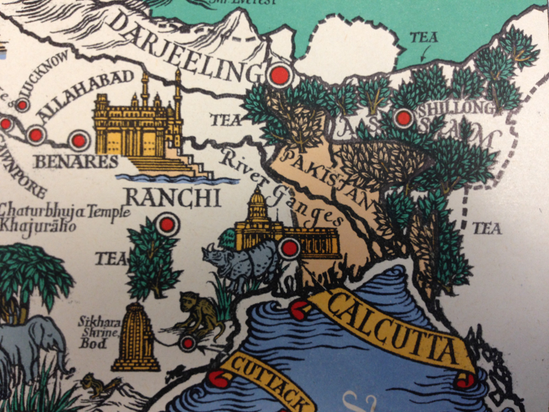
The Map Room is a pen-free zone; if you’re writing something, use a pencil. Smartphones and hand-held cameras are allowed, but under UL policy photos cannot be taken of the building itself. With prior permission however, it is possible to take images of material in the UL, which I did. The first series is from a map on display in the UL; titled “A map containing the towns villages gentlemen’s houses roads river and other remarks for 20 miles around London“, it was printed for a William Knight in 1710 and is a wonderful piece of cartography. The second series is from a map I requested using the card-index system; this map dates back to 1949 and beautifully illustrates tea-growing regions in the Indian-subcontinent.

If there’s a map in the UL you want an image of (for non-commercial or private-study purposes only!), I’d be happy to do what I can to help; I would actually be very grateful for an excuse to spend an afternoon looking at maps.


Using data from the Landsat 8 TIRS instrument to estimate surface* temperature

The Thermal InfraRed Sensor (TIRS) is a new instrument carried onboard the Landsat 8 satellite that is dedicated to capturing temperature-specific information.  Using radiation information from the two electromagnetic spectral bands covered by this sensor, it is possible to estimate the temperature at the Earth’s surface (albeit at a 100m resolution, compared to the 30m resolution of the other instrument, the Operational Land Imager).

The city-state of Delhi, India as visualised from band 10 of Landsat 8's TIRS instrument.

The city-state of Delhi, India as visualised from band 10 of Landsat 8's TIRS instrument.

I used data from the TIRS to estimate the surface temperature in the city-state of Delhi, India as of the 29th of May, 2013.  The relevant tarball file containing the data was downloaded using the United States’ Geological Survey’s (USGS) EarthExplorer tool; the area of interest was encompassed by [scene identifier: path 146 row 040] in the WRS-2 scheme. I think I’ll leave the specific explanations describing WRS-2, path/row values and the other miscellaneous small data-management operations for a later post. For now, I’ll just explain that these are important things to know when in the process of actually obtaining this data. When the tarball is unpacked fully, the bands from the TIRS instrument are bands 10 and 11;  the relevant .tif files are [“identifier”_B10.tif] and [“identifier”_B11.tif], and these were clipped to the administrative boundary of Delhi. There’s also a text file containing metadata: [“identifier”_MTL.txt] is essential for the math we’re going to do on these two bands. 

Each pixel of processed Level 1 (L1) Landsat 8 ETM+ data is stored as a Digital Number (DN) with a value between 0 and 2^15** . This means that when you visualise the two TIRS bands in your GIS/image-manipulation program of choice, you’re going to see a grey-scale image, where dark is cool and white is hot. The bands differ very slightly from each other; this is because each registers a different band of radiation, which is useful for correcting for atmospheric distortions.

To obtain actual surface temperature information, we need to first a) convert these DNs to top-of-the-atmosphere (ToA) radiance values, and then secondly b) convert the ToA radiance values to ToA brightness temperature in Kelvin.  The interesting thing is that the satellite stores information as radiance values; it’s converted to DNs when processed from L0 (raw data) to L1. We’re essentially reconverting this information to its original format.

Since the math does get a bit technical, I've posted the details at the end of this blogpost.

Since the TIRS has two bands, I conducted the mathematical operation on both, and then averaged the results. I know that there are more sophisticated ways of using both bands to accurately estimate surfacte temperature; as the USGS comment to this post has noted, I’ve only derived ToA brightness temperature here. Another step is required to calculate the actual surface temperature. In fact, a fellow Landsat 8 data user, Valerio de Luca, has informed me that there’s an equation of the split-window algorithm quadratic form that can be used for this purpose; thank you! I’ll update this post again once I test that. Finally, the conversion from degrees Kelvin to degrees anything else has been sufficiently well-documented that I’m going to leave it out; I’ve converted this map into degrees Celsius.

AvgTemp_Delhi-854x1024.jpg

An optional step in the middle is to correct for atmospheric distortion and solar irradiance by converting the DNs to ToA planetary reflectance values and then converting these to ToA radiance values. This requires information such as Earth-Sun distance and the solar angle, some of which is in the metadata file. I’ll be experimenting with this later as well.

Please pitch in if you have any suggestions on improving these techniques; I would definitely welcome points on better ways to use data from the TIRS instrument!

*Update 1 (245am IST on the 9th of August) : Firstly, I’d like to thank the USGS Landsat team, who’ve commented on this post; I’m very grateful for their encouragement and have updated the post accordingly. Please read the map title as ToA brightness-temperature in Delhi; another step is required before it accurately depicts the actual surface temperature values.

**Update 2 (2105 GMT on the 2nd of November) – Landsat 8 ETM+ Digital Number range has been corrected to reflect the fact that the ETM+ sensor stores 16-bit data; thanks for the comment Ciprian!

***Update 3 (0110 IST on the 5th of November 2017) - This article has been cross-posted from geohackers.in

I’ve referred to the documents below while figuring the math and writing this blogpost; they’re very useful.

USGS equations re: Landsat 8 data

https://landsat.usgs.gov/Landsat8_Using_Product.php

Converting Digital Numbers to Kelvin

http://www.yale.edu/ceo/Documentation/Landsat_DN_to_Kelvin.pdf

Information re: ToA reflectance

http://www.pancroma.com/Landsat%20Top%20of%20Atmosphere%20Reflectance.html

GRASS methodology

http://grass.osgeo.org/grass64/manuals/i.landsat.toar.html

More information on the inverted Planck function

http://www.yale.edu/ceo/Documentation/ComputingThePlanckFunction.pdf

Markham et al. (2005): Processing data from the EO-1 ALI instrument

http://www.asprs.org/a/publications/proceedings/pecora16/Markham_B.pdf

Converting from spectral radiance to planetary reflectance

http://eo1.usgs.gov/faq/question?id=21

<math>

a)             Digital Numbers to ToA radiance values

 = (ML * Qcal) + AL – - equation I

where:

Lλ        =          TOA spectral radiance

ML       =          Band-specific multiplicative rescaling factor

AL        =          Band-specific additive rescaling factor

Qcal        =        Quantized and calibrated standard product pixel values (DN)

Human-readable format:

Spectral Radiance = Band-specific multiplicative rescaling factor into Digital Number plus Band-specific additive rescaling factor from the metadata1. From the Markham et. al. (2005) paper on processing data from the EO-1 ALI instrument, I’m led to understand that the multiplicative and additive scaling factors result in ‘better preservaton of the ALI’s precision and dynamic range in going from raw to calibrated data’; this probably holds true for the L8 instruments as well but do correct me if I’m wrong.

In practise, this is:

[ Spec_rad_B“X”.tif ] = RADIANCE_MULT_BAND_”X”  * [“identifier”_B”X”.tif] + RADIANCE_ADD_BAND_”X”

where “X” is the specific band number, the RADIANCE values are obtained from the metadata file and Spec_rad_B”X”.tif is the output spectral radiance file name (user-determined).

b)            ToA radiance values to ToA brightness-temperature in Kelvin

T = K2 / (ln (K1/ Lλ +1))[2]   – equation II

(The physics-inclined will realise that equation II above is the inverted form of the Planck function.)

where:

T          =          ToA brightness temperature (K)
Lλ        =          TOA spectral radiance
K1        =          Band-specific thermal conversion constant
K2        =          Band-specific thermal conversion constant

 Human-readable format:

Temperature (Kelvin) = Band-specific thermal conversion constant I by the natural log of (Band-specific thermal conversion constant II by spectral radiance plus 1)

In practise, this is:

[Temp_B”X”.tif] = K2_CONSTANT_BAND_”X” / ln((K1_CONSTANT_BAND_”X” / [Spec_rad_B”X”.tif]) + 1)

where “X” is the specific band number, the CONSTANT values are extracted from the metadata file and the Temp_B”X”.tif file is the output temperature file name (user-determined).

 </math>

Landsat 8 data and maps of Delhi

This will be a relatively short post; I’ve been working with Landsat data for a few years now, and I find it absolutely fascinating. The new Landsat satellite, initially named the Landsat Data Continuity Mission and now known as Landsat 8, is actually the 7th in the series; Landsat 6 never made it to orbit. When Landsat 8 was launched on the 11th of February 2013, I was really anxious and excited and when it made it to orbit successfully, I was ecstatic. I downloaded my first set of Landsat data (Path146/Row040, covering the Indian city of Delhi) off the USGS EarthExplorer website last week, and have been tinkering with it ever since.

State_of_Delhi_L8_imagery-1024x724.jpg


The map above depicts various band-combinations; each band covers a discrete section of the electromagnetic spectrum. While bands 2, 3 and 4 lie within the visible spectrum and correspond to the colours blue, green and red, the others extend into the non-visible electromagnetic spectrum. A variety of mathematical operations can be conducted using different band combinations to obtain meaningful information about the Earth’s surface. For example, the following maps depict the surface temperature in Delhi, with a close-up of the Yamuna, on the 29th of May. A longer post on Landsat 8, its instrumentation and the various use-cases will follow once I’ve had my fill of playing with this data.